We’d like to share a simple modeling for predicting whether players will leave or not. We used R as an analysis tool, and the final model has F1-score of 0.4832.
We proceeded the modeling in the following order.
- Data Processing
- Data Visualization
- Data Modeling and Performance Comparison
- Measurement of final test results
- Data Processing
This is the stage where features for the model are created and integrated with the game log data of each account. The data provided were as follows.
| Data Set | Sample Size | Period (8 weeks) | ||
|---|---|---|---|---|
| churn = 1 | churn = 0 | total | ||
| Train | 1,200 | 2,800 | 4,000 | 2016-03-16 06 ~ 2016-05-11 06 |
| Test1 | 900 | 2,100 | 3,000 | 2016-07-27 06 ~ 2016-09-21 06 |
| Test2 | 900 | 2,100 | 3,000 | 2016-12-14 06 ~ 2017-02-28 06 |
First, we created a feature that would affect players’ leaving. There are four types of features.
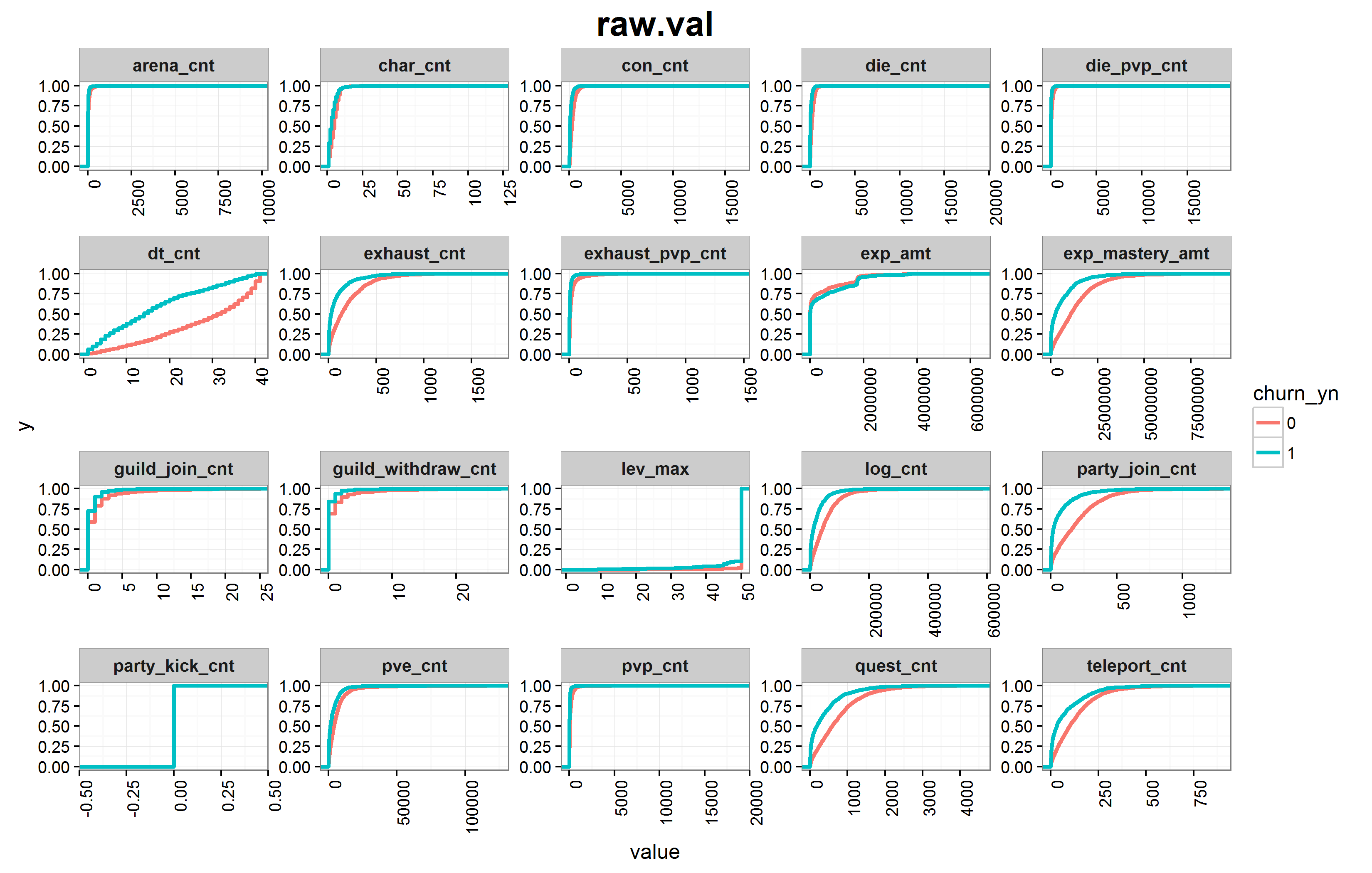
√ raw.val: This is a total count or amount in the period. That is, it shows the amount of usage per feature for 8 weeks.
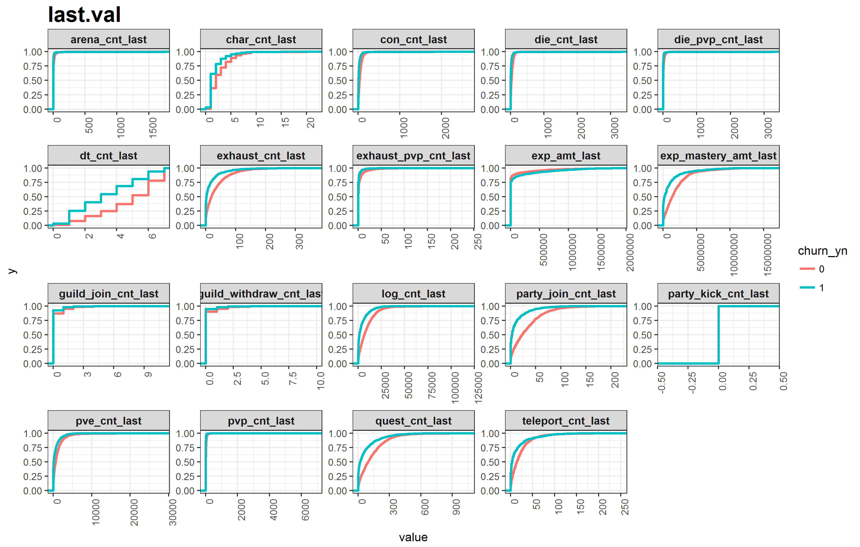
√ last.val : This is the final week’s count or amount in the same period. It is based on the assumption that the most recent playing will affect the churning.
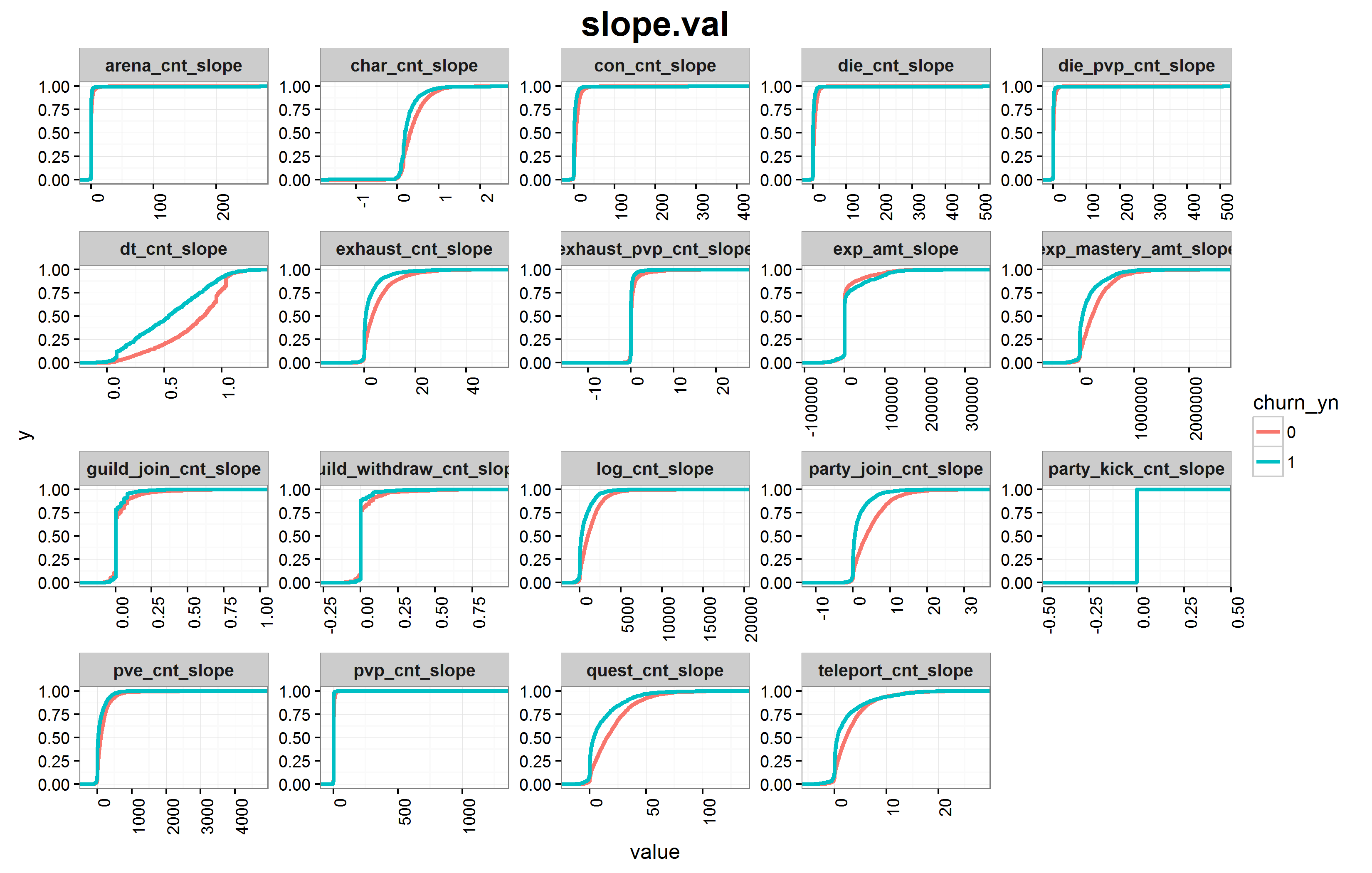
√ slope.val : This is a slope value of the simple linear regression model for each weekly usage. It is based on the assumption that the amount of usage will decrease as it gets closer to the time of a leave.
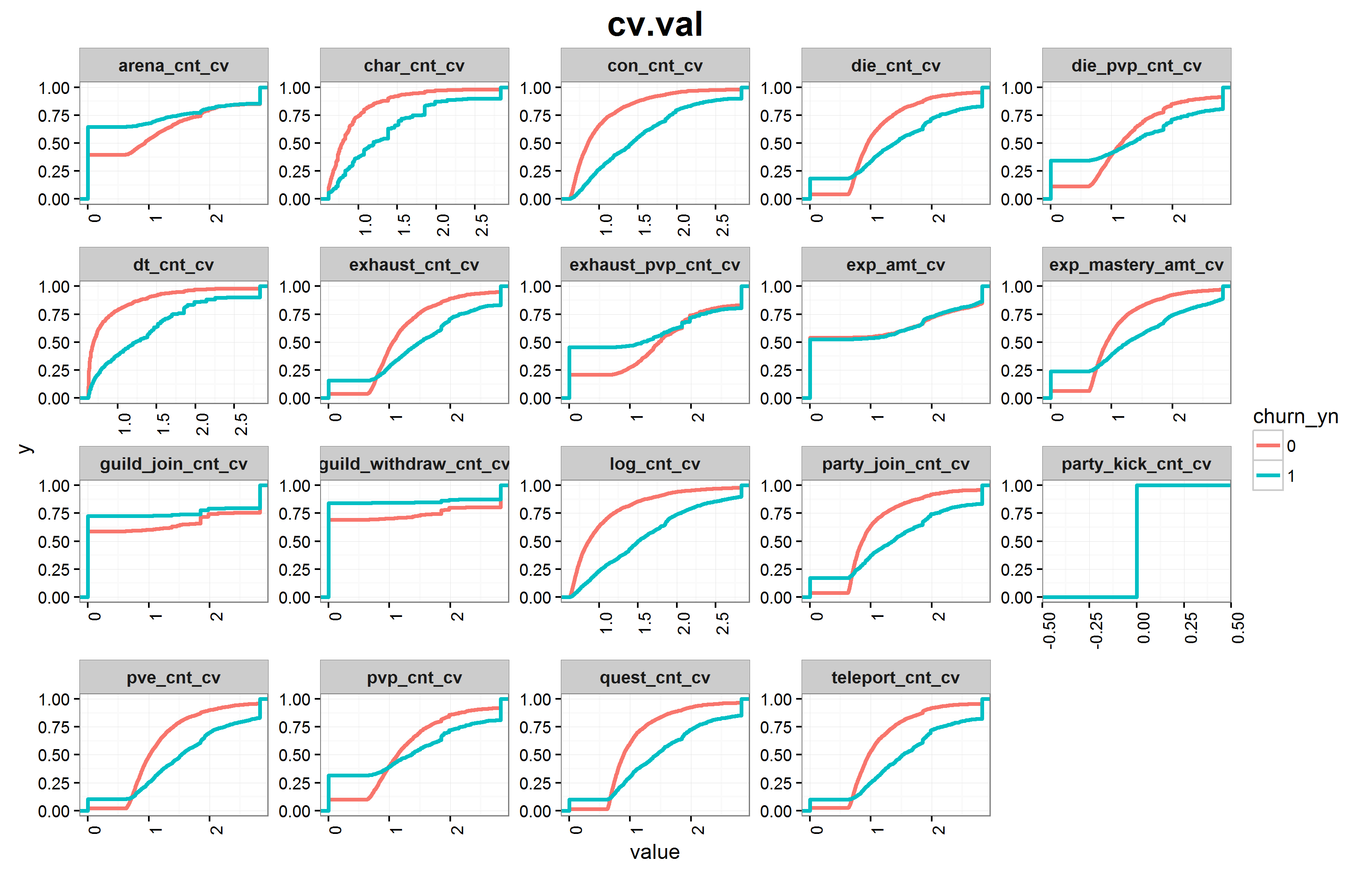
√ cv.val : Coefficient of variation for each weekly usage. It is based on the assumption that players who play infrequently are more likely to leave than to steadily play.
The generated variable list is as follows.
| no. | feature | type | |||
|---|---|---|---|---|---|
| raw.val | last.val | slope.val | cv.val | ||
| (1) | dt_cnt | O | O | O | O |
| (2) | con_cnt | O | O | O | O |
| (3) | log_cnt | O | O | O | O |
| (4) | char_cnt | O | O | O | O |
| (5) | exp_amt | O | O | O | O |
| (6) | exp_mastery_amt | O | O | O | O |
| (7) | exhaust_cnt | O | O | O | O |
| (8) | exhaust_pvp_cnt | O | O | O | O |
| (9) | die_cnt | O | O | O | O |
| (10) | die_pvp_cnt | O | O | O | O |
| (11) | quest_cnt | O | O | O | O |
| (12) | party_join_cnt | O | O | O | O |
| (13) | party_kick_cnt | O | O | O | O |
| (14) | teleport_cnt | O | O | O | O |
| (15) | pve_cnt | O | O | O | O |
| (16) | pvp_cnt | O | O | O | O |
| (17) | arena_cnt | O | O | O | O |
| (18) | guild_join_cnt | O | O | O | O |
| (19) | guild_withdraw_cnt | O | O | O | O |
| (20) | char_lev_max | O | |||
| (21) | char_lev_job | O | |||
| (22) | guild_char_cnt | O | |||
(1) dt_cnt : the number of logged-in days
(2) con_cnt : the number of times player have entered the world (Logid = 1003)
(3) log_cnt : the number of generated logs
(4) char_cnt : the number of characters played
(5) exp_amt : the total amount of experience acquired while playing
(6) exp_mastery_amt : the total amount of mastery-experience acquired while playing
(7) exhaust_cnt: the number of times a player has exhausted (Logid = 1201)
(8) exhaust_pvp_cnt : the number of times a player is exhausted by another player (logid = 1201 and target_code = 10)
(9) die_cnt : the number of times a player has fainted or died (Logid = 1202)
(10) die_pvp_cnt : the number of times a player has fainted or died by another player (Logid = 1201 and target_code = 10)
(11) quest_ cnt : the number of completed quests (Logid = 5004)
(12) party_join_cnt : the number of party participation (Logid = 1102)
(13) party_kick_cnt : the number of times a player banned from a party (Logid = 1106)
(14) teleport_cnt : the number of teleports (Logid = 1010)
(15) pve_ cnt : the number of PvE times (Logid = 1208) cf. PvE means a player killing an NPC.
(16) pvp_ cnt : the number of PvP times. (Logid = 1209) cf. PvP means a player killing a PC.
(17) arena_cnt : the number of times when a team or individual duel has ended (Logid = 1404, 1406)
(18) guild_join_cnt : the number of times a player joining a clan. (Logid = 6005)
(19) guild_withdraw_cnt : the number of times a player quitting a clan. (Logid = 6009)
(20) char_lev_max : the highest level of a character. The maximum value of the ‘actor_level’ field.
(21) char_lev_job : the job of a character with the highest level and the highest log volume among characters played.
(22) guild_char_cnt : the number of characters who have joined a clan.
The query that extracts variables of type raw.val using R is as follows.
| raw.val <- sqldf(” select actor_account_id , count(distinct nc_dt) as dt_cnt , count(case when logid = 1003 then 1 end) as con_cnt , count(1) as log_cnt , count(distinct actor_id) as char_cnt , count(case when logid = 1016 then use_value1_num end) as exp_amt , count(case when logid = 1016 then use_value3_num end) as exp_mastery_amt , count(case when logid = 1201 then 1 end) as exhaust_cnt , count(case when logid = 1201 and target_code = 10 then 1 end) as exhaust_pvp_cnt , count(case when logid = 1202 then 1 end) as die_cnt , count(case when logid = 1202 and target_code = 10 then 1 end) as die_pvp_cnt , count(case when logid = 5004 then 1 end) as quest_cnt , count(case when logid = 1102 then 1 end) as party_join_cnt , count(case when logid = 1106 then 1 end) as party_kick_cnt , count(case when logid = 6005 then 1 end) as guild_join_cnt , count(case when logid = 6009 then 1 end) as guild_withdraw_cnt , count(case when logid = 1010 then 1 end) as teleport_cnt , count(case when logid = 1208 then 1 end) as pve_cnt , count(case when logid = 1209 then 1 end) as pvp_cnt , count(case when logid in (1404, 1406) then 1 end) as arena_cnt from data group by actor_account_id “)temp <- sqldf(” select actor_account_id, actor_job, max(actor_level) as lev_max, count(1) as log_cnt from data group by actor_account_id, actor_job order by actor_account_id, lev_max_Desc, log_cnt desc “) raw.val$char_lev_max <- temp[1, 3] raw.val$char_lev_job <- temp[1, 2]temp <- sqldf(” select actor_account_id, count(distinct a.actor_id) as guild_char_cnt from ( select actor_account_id, actor_id, actor_guild, actor_job from data where actor_guild > 0 group by actor_account_id, actor_id, actor_guild, actor_job ) a left outer join ( select actor_account_id, actor_id, actor_guild, actor_job from data where logid = 6009 group by actor_account_id, actor_id, actor_guild, actor_job ) b on a.actor_id = b.actor_id and a.actor_guild = b.actor_guild where b.actor_guild is null “) |
The following time table is created considering a week starts from Wednesday, 6:00 a.m. to the next Wednesday, 6:00 a.m. The weekly and daily counts were calculated based on the weeks(bs_wk) and days(bs_dt).
| bs_wk | bs_dt | time_from | time_to |
|---|---|---|---|
| 201612 | 20160316 | 2016-03-16 6:00 | 2016-03-17 6:00 |
| 201612 | 20160317 | 2016-03-17 6:00 | 2016-03-18 6:00 |
| 201612 | 20160318 | 2016-03-18 6:00 | 2016-03-19 6:00 |
| 201612 | 20160319 | 2016-03-19 6:00 | 2016-03-20 6:00 |
| 201612 | 20160320 | 2016-03-20 6:00 | 2016-03-21 6:00 |
| 201612 | 20160321 | 2016-03-21 6:00 | 2016-03-22 6:00 |
| 201612 | 20160322 | 2016-03-22 6:00 | 2016-03-23 6:00 |
| 201613 | 20160323 | 2016-03-23 6:00 | 2016-03-24 6:00 |
| … | … | … | … |
- Data Visualization
We visualized the features and looked for the differences depending on whether players leaves or not. The graph below shows the cumulative distribution function of each feature. As you can see, there exist features with differences between the leaving and non-leaving groups.
- Data Modeling and Performance Comparison
We used Random Forest, SVM, and Lasso Regression for Model Generation. For the final model selection, Train set was divided into 70:30. 70% was used for Model Learning, and 30% was used for Performance Measurement.
- AUC
| Random Forest | 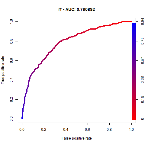 |
| Support Vector Machine | 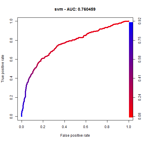 |
| Lasso Regression |  |
- Confusion matrix
b-1. Random Forest
| F1-score : 0.6079 Accuracy : 0.7084 |
Actual value | ||
|---|---|---|---|
| 1 | 0 | ||
| Predicted value | 1 | 262 | 240 |
| 0 | 98 | 559 | |
b-2. Support Vector Machine
| F1-score : 0.5798 Accuracy : 0.7606 |
Actual value | ||
|---|---|---|---|
| 1 | 0 | ||
| Predicted value | 1 | 198 | 125 |
| 0 | 162 | 714 | |
b-3. Lasso Regression
| F1-score : 0.6094 Accuracy : 0.7306 |
Actual value | ||
|---|---|---|---|
| 1 | 0 | ||
| Predicted value | 1 | 252 | 215 |
| 0 | 108 | 624 | |
- Measurement of final test results
After the performance evaluation using Random Forest, SVM and Lasso Regression, the test set prediction was finally performed by the lasso model as the final model. The final result of the comparison between the predicted value and the actual value of the test data is as follows.
| Test1 score | Test2 score | Total score |
|---|---|---|
| 0.4982 | 0.4691 | 0.4832 |